This post is another in a series I've done on the SIM model described by Godley and Lavoie (G&L) in Chapter 3 of their book
Monetary Economics [
pdf]. I refer to G&L's original discrete time version of the model as $SIM_d$ and I introduce here a continuous time version of it that I refer to as $SIM_c$. $SIM_c$ is different from the continuous time versions I've discussed in my SIM8 and earlier posts (e.g. $SIM_m$), though it is related to the concepts I introduce in SIM9. The other main purpose of this post is to implement $SIM_c$ as an interactive circuit model so you can see it in action, and see how it relates to $SIM_d$.
This post (like several other of my recent SIM posts) is related to a post by
Jason Smith on SFC models. I also credit
Roger Sparks for stoking my interest in this circuit analogy and for providing feedback.
Update Start: 2016.04.20 10:53 AM
I simplified the Y(t) charge (=voltage across 1-F capacitors) output by consolidating the Yodd(t) and Yeven(t) by adding another switch, and I stacked it on top of the y(t) current plot so you can more easily see the time relation between SIM outputs (peaks of Y(t) "saw-teeth") and the underlying continuous model here (which produces y(t)). I also added a way to easily adjust g(t) (the instantaneous government gross spending rate) once the the simulation starts (i.e. once you close the activation switch (top-center)): it still defaults to 20 dollars per unit time, but now you can adjust it while the simulation is running via the slider in the right side-bar labeled "Voltage" (under the other sliders such as "Current Speed" etc). Here's the new URL (in its "tinyurl" format -- the other is ~4241 characters long, and exceeds blogger's allowed comment size!):
https://tinyurl.com/yc86aun6 (and the "preview" version: http://preview.tinyurl.com/yc86aun6). Also, here a screen capture with annotations (figure 0: click to enlarge):
 |
| Figure 0: Updated simulation screen capture with annotations (click to enlarge) |
Feel free to edit them however you like: you can't mess up the original (and if you want start over, just refresh your browser). If you want to store your creation, use the file menu. See
the extended table of Godley & Lavoie's (G&L) SIM results (with
default parameters) near the bottom of this post, and compare with the
peak values produced in the curve Y(t) (lower left scope, top (green)
trace). The simulation value in white text in the upper right of each
scope trace (scopes are along the bottom) records the value of the
highest peak of that trace, so this value will persist until another
larger peak is encountered, giving you time to pause the simulation
(with the "Stopped" check box in the right side-bar) to do the
comparison.
Update End: 2016.04.20 10:53 AM
This post discusses several electric circuit representations of SIM,
especially this implementation using operational amplifiers (op amps) which partially bridges the gap between the continuous time and discrete time models (with only a single "flow" variable ($Y$).
This comment I left on Nick Edmond's blog is a pretty good summary.
Money is modeled as coulombs with 1 coulomb = 1 dollar. Sample periods ($T_s$) are modeled as seconds. After clicking on the link, activate the circuit by clicking on the switch at the top, as shown in figure 1 (click on figure 1 to get a more detailed view). After the activation switch changes from ground to +5 volts, it may take it a short while before the next rising clock edge actually activates the circuit. This is done to synchronize the integration of $y(t)$ in with the ping pong integrators so that the outputs of these integrators match G&L's values of $Y$ in their table. Check the outputs ($Y_{odd}$ and $Y_{even}$) when they reach their peak at the end of each integration interval (in the lower right corner). I had to divide it into a pair of ping-poing integrators because a single integrator didn't discharge fast enough so as not to confuse the circuit simulator. In principal, this same technique could be applied to generate $T, Y_D, C$ and the input $G$ so that they all match G&L's table. $H$ will already match, since $H(t)$ is a stock, integrated from $t = -\infty$ rather than a sliding integral over just the last sample period.
The instantaneous curves will all satisfy G&L's accounting identities over any sample period, not just at the sample times G&L have chosen in their example. You can think of this as the instantaneous values ($g(t), y(t), \tau (t), y_D (t)$ and $c(t)$) being valid "flows" over infinitesimally small sample intervals.
 |
| Figure 1: Screen shot of SIM implemented with instantaneous equations in op amp circuit with sliding window integration to calculate "flows" (click on to enlarge) |
This post borrows heavily from
a previous page I put up here with other circuit implementations of parts of SIM, but also from the
2016.04.18 update to SIM9. On that previous page with circuit implementations of SIM I touched on doing a full circuit implementation of SIM using a circuit with operational amplifiers (op amps) in comments dated 2016.04.17. I did produce such an implementation for the case of outputs corresponding to G&L SIM discrete time outputs ($Y, T, Y_D$ and $C$) and the SIM discrete time input ($G$) all of which represent integrated values of some underlying finer grain discrete time function or an integration of some underlying continuous time function. There are an infinite number of such underlying discrete time or continuous time functions which would map to SIM's sampled output values, but in the case of continuous time models, there's one model in particular that suggests itself as the simplest. In that simple continuous time model, the values $G, Y, T, Y_D$ and $C$ represent samples from continuous time functions, which themselves are sliding window integrals (over a window of time equal to the length of 1-sample period = $T_s$) of other continuous time functions representing
instantaneous rates, all in dollars per unit time. My post SIM 9 discusses this further.
Equations to define a continuous time version of SIM using instantaneous flows:
The
following are the equations for the continuous time
state space
matrices we've chosen to implement here in terms of their (original)
discrete time counterparts:
$$A_c = \frac{1}{T_{s_0}} \ln (A_d)\tag {1a}$$
$$B_c = \frac{A_c}{Ad - 1} T_{s_0} B_d \tag {1b}$$
$$C_{c} = \frac{A_c}{A_d -1} C_d \tag 2$$
$$D_{c} = \frac{A_c T_{s_0} + 1 - A_d}{(A_d - 1)^2} B_d C_d + D_d = \frac{B_c - B_d}{A_d - 1} C_d + D_d \tag 3$$
The "d" subscript indicates discrete time while the "c" subscript indicates continuous time. In this case $A_d, B_d, A_c, B_c \in ℝ^{1 \times 1}$ (i.e. they are real valued scalars), while $C_d, D_d, C_c, D_c \in ℝ^{4 \times 1}$ (i.e. they are real valued $4 \times 1$ columns vectors). $T_{s_0}$ is the default (original) SIM sample period and is implicitly
defined as "1 period" (i.e. with numerical value 1 unit of time) in G&L's
description of SIM. I always call it the default (or original) sample
period because the continuous time model is independent of whatever
sample period ($T_s$) we choose, but it's defined in terms of a discrete
time model (the original SIM model) which itself is defined in terms of
an original sample period ($T_{s_0}$).
These results could probably be generalized to cases with more than one state (i.e. $A_d, A_c \in ℝ^{N \times N}$) by replacing $1/(A_d - 1)$ with $(A_d - I)^{-1}$ and of course replacing the scalar multiplies by matrix multiplies (where appropriate), at least in cases where $A_d - I$ is invertible. The fact that $A_c A_d = A_d A_c$ should help with that (see the
definition of a matrix exponential for why that is [and notice that $A_d = e^{A_c T_{s_0}}$]). I'd guess it can probably also be done for cases where $A_d - I$ is not invertible (i.e. it's singular) with some mess involving
Jordan blocks or some such.
Keep in mind that the particular continuous time system we've chosen here is not unique, and there are an infinite number of other possible choices. Also keep in mind that the discrete time system (in this case) is not simply samples of an underlying continuous time system (as is the case in may other discrete-time continuous-time pairs, for example in many engineering applications). Instead the discrete time system represents the outputs of a series of "accounting intervals" over which continuous time rate variables (which I sometimes refer to as "instantaneous flows") (measured in dollars per unit time) must be integrated to produce values comparable with the corresponding flow values produced by the discrete time model. Essentially, the sampling is done at the end of this accounting (integration) procedure over each period. This is the reason that $C_c \neq C_d$ and $D_c \neq D_d$ in this case, unlike in many engineering applications, where the measurement (or output) matrix ($C$) and feed-through (or feed-forward) matrix ($D$) are equal to their discrete time counterparts. That's because in those engineering applications, the instantaneous rates (in constant units) are what we're typically interested in (both in continuous time and discrete time), rather than their integrals over each sample period. Because of this dependence on integrating over sample intervals in SIM, then as $T_s \rightarrow 0$ all the SIM flow values $\rightarrow 0$ as well (i.e. $G, Y, T, Y_D, C \rightarrow 0$). In contrast, the "instantaneous flows" $g, y, \tau, y_D, c \nrightarrow 0$ as $T_s \rightarrow 0$ because they are independent of the sample period ($T_s$) chosen.
[To do: show how I derived the above equations]
[To do: show a closed form means of using these result to change the sample period like in SIM1, SIM2, SIM3 and SIM6] Done (see equations (i) through (iv) below).
Op amp circuit simulation parameter (i.e. resistor) values
For the following explanation related to the below tables,
refer to equations $(4), (5), (6), (13), (14)$, and $(15)$ in the
section below this one. Given an instantaneous flow input $g(t)$ (in amperes := coulombs per second) the circuit produces instantaneous flow outputs $y(t), \tau (t), y_D (t)$ and $c(t)$ also in amperes. Integrating these instantaneous flows over each default SIM sample period of length $T_{s_0}$ produces values of charge in coulombs (equivalent to volts across the 1-F capacitors used) which are numerically equivalent to corresponding SIM flow values $G, Y, T, Y_D$ and $C$ in dollars over the period. It also produces an instantaneous stock $H(t)$ in coulombs of charge (again measurable in volts across the 1-F capacitor used), which at the default sample times is equivalent to the SIM stock value $H$ in dollars.
| Table
1: SIM Parameters |
| Symbol |
Value |
| $T_{s_0}$ |
1 |
| α1 |
0.6 |
| α2 |
0.4 |
| θ |
0.2 |
| Table
2: Useful Expressions |
| Name |
Expression |
Value |
| P |
1 - α1(1-θ) |
0.52 |
| $Q$ |
$A_c/(A_d-1)$ |
1.085852 |
| $V$ |
$(B_c-B_d)/(A_d-1)$ |
-0.34341 |
 |
| Figure 0a: Detail of figure 0: parameter resistors |
| Table
3: Discrete Time State Space Matrices ($SIM_d$) |
| Matrix |
Elements |
Name |
Expression |
Value |
| $A_d$ |
$A_{d_{1,1}}$ |
$A_d$ |
1 - α2θ/P |
0.84615385 |
| $B_d$ |
$B_{d_{1,1}}$ |
$B_d$ |
1 - θ/P |
0.61538462 |
| $C_d$ |
$C_{d_{1,1}}$ |
$C_Y$ |
α2/P |
0.76923077 |
| $C_{d_{2,1}}$ |
$C_T$ |
α2θ/P |
0.15384615 |
| $C_{d_{3,1}}$ |
$C_{Y_D}$ |
α2(1-θ)/P |
0.61538462 |
| $C_{d_{4,1}}$ |
$C_C$ |
α2/P |
0.76923077 |
| $D_d$ |
$D_{d_{1,1}}$ |
$D_Y$ |
1/P |
1.92307692 |
| $D_{d_{2,1}}$ |
$D_T$ |
θ/P |
0.38461538 |
| $D_{d_{3,1}}$ |
$D_{Y_D}$ |
(1-θ)/P |
1.53846154 |
| $D_{d_{4,1}}$ |
$D_C$ |
α1(1-θ)/P |
0.92307692 |
| Table
4: Continuous Time State Space Matrices ... |
... and Resistors |
| Matrix |
Elements |
Name |
Expression |
Value |
Name |
Expression |
Value (Ω) |
| $A_c$ |
$A_{c_{1,1}}$ |
$A_c$ |
$\ln(A_d)/T_{s_0}$ |
-0.16705 |
$R_a$ |
$-{A_c}^{-1}$ |
5.986085 |
| $B_c$ |
$B_{c_{1,1}}$ |
$B_c$ |
$Q T_{s_0} B_d$ |
0.668216 |
$R_b$ |
${B_c}^{-1}$ |
1.496521 |
| $C_c$ |
$C_{c_{1,1}}$ |
$C_y$ |
$Q C_d$ |
0.83527 |
$R_{C_y}$ |
${C_y}^{-1}$ |
1.197217 |
| $C_{c_{2,1}}$ |
$C_{\tau}$ |
0.167054 |
$R_{C_{\tau}}$ |
${C_{\tau}}^{-1}$ |
5.986085 |
| $C_{c_{3,1}}$ |
$C_{y_D}$ |
0.668216 |
$R_{C_{y_D}}$ |
${C_{y_D}}^{-1}$ |
1.496521 |
| $C_{c_{4,1}}$ |
$C_c$ |
0.83527 |
$R_{C_c}$ |
${C_c}^{-1}$ |
1.197217 |
| $D_c$ |
$D_{c_{1,1}}$ |
$D_y$ |
$V C_d + D_d$ |
1.658918 |
$R_{D_y}$ |
${D_y}^{-1}$ |
0.602802 |
| $D_{c_{2,1}}$ |
$D_{\tau}$ |
0.331784 |
$R_{D_{\tau}}$ |
${D_{\tau}}^{-1}$ |
3.014012 |
| $D_{c_{3,1}}$ |
$D_{y_D}$ |
1.327135 |
$R_{D_{y_D}}$ |
${D_{y_D}}^{-1}$ |
0.753503 |
| $D_{c_{4,1}}$ |
$D_c$ |
0.658918 |
$R_{D_c}$ |
${D_c}^{-1}$ |
1.517639 |
Table 4 (above) shows the resistor values in ohms (Ω) needed to implement (via the op amp circuit) the version of the
continuous time circuit described in this post. The resistors are labeled in
figure 0 to match the red colored values in the right most column.
Figure 0a to the right shows a detail of figure 0, so the pertinent
resistor labels are easier to read. Table 1 shows the original discrete time SIM model's parameters. Table 2 defines some useful expressions. Table 3 translates the original discrete time SIM (call that model $SIM_d$) parameter values into a set of state space matrices. There's an interactive embedded spreadsheet version of tables 1 through 4 on this page.
Note that the version of the continuous time system implemented here produces instantaneous "flow" (i.e. instantaneous rate values) (in dollars per unit time) which correspond to the original discrete time SIM flow variables. SIM8 equation $(2)$ gives another version of a continuous time system (the continuous time state space matrices there are subscripted with "m" instead of "c"), the samples of which themselves match the discrete time SIM if $T_s = T_{s_0}$. The instantaneous flows in this version of continuous time SIM (unlike the stock variable $H(t)$, which is the same for SIM8 $(2)$ and here because $A_c = A_m$ and $B_c = B_m$) must be integrated over a sample period to recreate the corresponding SIM flow variables. These instantaneous flow values will NOT match SIM outputs without doing this integration. However, integrating these flows over any arbitrary time interval should produce results which obey G&L's accounting identities, which is not the case with SIM8 $(2)$. Note that $SIM_m$ could also be constructed with the op amp circuit presented here by using $A_c$ and $B_c$ from table 4 and $C_d$ and $D_d$ from table 3 as the basis of calculating the resistor values. If this were done, the ping-pong integrators should be removed or ignored.
The instantaneous stock variable $H(t)$ is the same for the continuous time model presented here (call that model $SIM_c$) and for the one in SIM8 $(2)$ (call that model $SIM_m$). That's because $A_c = A_m$ and $B_c = B_m$. In both cases $H(t)$ matches the $SIM_d$ stock variable $H$ once the indexing depicted in figure 2 (below) is taken into account. That's because the continuous time flow variables in $SIM_m$ are directly representing the sample-period integrated instantaneous flows modeled in $SIM_c$, provided the sample period is $T_{s_0}$ and that the sample times coincide with those of $SIM_d$. $SIM_m$ stock and flow values are not guaranteed to satisfy G&L's accounting equations for other sample periods or sample times.
Using the continuous time SIM with instantaneous flows to find new discrete time models with arbitrary sample periods (i.e. how to change the sample period):
Changing the sample periods has been one of my primary goals with this series of posts since SIM1, and in fact versions of this concept are implemented in SIM1, SIM2, SIM3 and SIM6. How will this approach differ? Well here I'm not attempting to change the sample period for the model $SIM_c$ since that model is independent of the sample times (and actually has no sample times). However, a discrete time model which is the product of integrating the instantaneous flows of $SIM_c$ over each sample period, and then sampling at the end of each integration (at the end of each sample period ($T_s$), when the output of the integration has reached a peak) will be dependent on sample times, and thus it makes sense to speak of adjusting it for the sample period. Let's call this resultant discrete time model $SIM_{T_s}$ to indicate that it's sample period is $T_s$, and let's call its output matrix $C_{T_s}$ and its feedthrough matrix $D_{T_s}$. Here are some things we know about such a discrete time model, which we can use to check our work:
- When $T_s = T_{s_0}$ it reduces to the original $SIM_d$ model.
- At $T_s = 0$ the flows of $SIM_{T_s}$ will also be $0$ since the
integration time will be $0$, and thus $C_{T_s} = 0$ and $D_{T_s} G_n = 0$. Keep in mind also that as $T_s \rightarrow 0,\; G_n \rightarrow 0,\;\forall n$ since $G$ is also a flow, and as the integration window $T_s$ drops to $0$ so does $G_n$ (unless of course it contains Dirac delta functions).
- $d C_{T_s} / d T_s$ evaluated at $T_s = 0$ will be equal to $C_c$
and $d (D_{T_s} T_s) / d T_s$ evaluated at $T_s = 0$ will be equal to $D_c$.
This is because $C_c$ and $D_c$ form the measurement equation for
instantaneous flows, which is what happens in the limit for flows over a
sample period $T_s$ as $T_s \rightarrow 0$. Again, keep in mind $G$ is also a flow.
- If as $t \rightarrow \infty,\; g(t) \rightarrow \overline{g} > 0$
(where $\overline{g} \equiv$ the steady state value of $g(t)$) then as
$T_s \rightarrow \infty$ we should have $SIM_{T_s}$ flows also going to
$\infty$ because we're integrating over an infinite window of the
non-zero steady sate of the model. Keep in mind also that if $g(t) \rightarrow \overline{g} > 0$ as $t \rightarrow \infty$ then we'll have $G_n \rightarrow \infty,\;\forall n$ because $G$ is also a flow, and is thus integrated over an unbounded sample period.
- If as $t \rightarrow \infty,\; g(t) \rightarrow \overline{g} > 0$
then as $T_s \rightarrow \infty$ we should have $SIM_{T_s}$ flows
averaged over an interval of length $T_s$ going to the steady state
value of the flows divided by $T_{s_0}$.
Given the above and our previous values for $SIM_c$ and $SIM_d$ system matrices we can find values for the system matrices of this new discrete time system $SIM_{T_s}$ as follows:
$$A_{T_s} = {A_d}^{T_s/T_{s_0}}\tag{i}$$
$$B_{T_s} = \frac{A_{T_s} - 1}{A_d - 1}\frac{T_{s_0}}{T_s} B_d\tag{ii}$$
$$C_{T_s} = \frac{A_{T_s} - 1}{A_d - 1} C_d\tag{iii}$$
$$D_{T_s} = \frac{A_{T_s} - 1 - A_c T_s}{(A_d - 1)^2} \frac{T_{s_0}}{T_s} B_d C_d + D_c\tag{iv} = \frac{\frac{T_{s_0}}{T_s}(A_{T_s} - 1) - (A_d - 1)}{(A_d - 1)^2} B_d C_d + D_d$$
See SIM2 and SIM6 for more information on $(\text{i})$ and $(\text{ii})$. Compare the first expression for $D_{T_s}$ in $(\text{iv})$ with the first expression for $D_c$ in $(3)$ above, and notice that substituting $D_c$ from $(3)$ into the first expression for $D_{T_s}$ in $(\text{iv})$ results in the second expression for $D_{T_s}$ in $(\text{iv})$ (because the $A_c$ terms cancel), which clearly is just $D_d$ when $T_s = T_{s_0}$ (since, by $(\text{i})$ $A_{T_s} = A_d$ when $T_s = T_{s_0}$).
 |
| Figure 3a: changing Ts during a run |
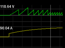
Figure 3a at the right shows the effects of changing the sample period
in the circuit on the fly by adjusting the frequency of the clock (CLK).
See figure 3 below for an explanation of the curves, but basically it's
Y(t) (green) above y(t) (yellow). Activity starts when the government
spending rate (not pictured) steps up (instantaneously) from 0 to 20 dollars per unit time at t=0 (precisely where y(t) steps up in figure 3a). The 1st couple of periods were set to 2 seconds
(corresponding to a clock frequency of 0.25 Hz), the middle four were at
1-second (the default, corresponding to a clock of 0.5 Hz) and the
final set were at a clock of 1-Hz giving a 0.5 second sample
(accounting) period. Notice how the peaks decrease in proportion to the
sample period, and that the sample period has no effect on the
instantaneous rate curve y(t).
I'm not sure what the relationship is between the discrete time model here ($SIM_{T_s}$) sampled at arbitrary sample period $T_s$ not necessarily equal to $T_{s_0}$ and the model presented in post SIM6 in which the original G&L discrete time SIM (i.e. $SIM_d$) parameters $\alpha_1$ and $\alpha_2$ were adjusted (along with the period labels in the spreadsheet) to produce a discrete time model which exactly preserved $SIM_d$'s steady state values and its "adjustment time" (i.e. time constant = $T_c$), while still obeying G&L's accounting identities over each period. I suspect they may be the same model, at least over some range of the parameters. However, I'm confident the model here can be used with any sample period without any issues, since I'm not explicitly changing any $SIM_d$ parameters (other than its implicit sample period of course). NOTE: I added tables 5 through 7 to the
interactive embedded spreadsheet here and discovered that the values produced for the system matrices for $SIM_{T_s}$ match those produced by the embedded spreadsheet in
post SIM6 (for an example with $T_s = 0.4$ and $T_{s_0} = 1$, but I still need to show a mathematical connection).
[To do: finish this section: explain the derivation of $(\text{i})$ through $(\text{iv})$, and show that they satisfy our expectations (1 through 5) for the solution. Also, double check this whole post to make sure I have my $T_{s_0}$ and $T_s$ and corresponding explanations correct in all parts. That gets confusing! Also, figure out if $SIM_{T_s}$ presented here is the same as the discrete time model presented in post SIM6.]
Relating G&L SIM stock and flow variables to a continuous time model with instantaneous rates:
I'm reluctant to bring this up yet again (see SIM4, SIM7 and SIM9), because I really struggle with trying to communicate this in a logical and consistent fashion without stumbling over variable names and notation, but I need to revisit what is meant by some of the variable names on my annotated op amp circuit screen captures above. There are three issues at stake:
- What I (and Brian Romanchuk) have called the "non-canonical" nature of SIM's iterative equations in comparison with a "canonical" state space expression.
- What G&L's "periods" are and how they relate to a "normal" discrete time or continuous time timeline
- What I've referred to as the "average vs instantaneous" continuous time equivalent "flow" variables (in the sense of stocks and flows in stock flow consistent (SFC) models).
I don't expect I will do a much better job here than I've done before, but I will try to limit the scope and only describe what I need to in order to fill in the gaps in the diagrams. It may change in the future, but not until the diagrams above change as well. First I need to relate what G&L call a "Period" in their Table 3.4 to a continuous time timeline. Figure 2 depicts how I'm choosing to understand the relation. It's unfortunate that G&L didn't call their "Period 1" "Period 0" instead, but oh well.
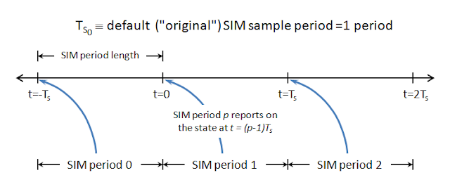 |
| Figure 2: SIM periods and how they relate to sample times and the continuous time timeline |
I feel the need to introduce the concept of a "default SIM sample period" or "original SIM sample period" which I call $T_{s_0}$ only because so many of my previous SIM posts (e.g. SIM1, SIM2, SIM3, SIM6) were concerned with altering this sample period. I don't get into that much in this post, so you can take $T_{s_0} = T_s \equiv \text{$``$the SIM sample period$"$}$ in this post, and further you can take the numerical value of $T_s$ to be $1$ (i.e. $1$ default SIM sample period). Of course SIM is presented as a discrete time model from the get go by G&L, so they aren't really sampling anything, but because my purpose here it to relate this model to an example of a continuous time model which is "equivalent" in some sense, I need to introduce the concept of sampling this underlying continuous time model.
As stated above, life would be slightly easier if G&L had chosen to name their initial period "Period 0" instead of "Period 1." An issue related to this is the "non-canonical" nature of the resulting discrete time "state space" system equations which can be written to represent SIM. These equations are:
$$H_{p+1} = A_d H_p + B_d G_{p+1} \tag 4$$
$$W_{p+1} = C_d H_p + D_d G_{p+1} \tag 5$$
where $A_d, B_d, C_d$ and $D_d$ are the usual state space system matrices for a discrete time linear time-invariant (LTI) system (the $d$ subscript here denoting discrete time). In this case, $H$ is the only state, thus $A_d \in ℝ^{1 \times 1}$ [1] (i.e. $A_d \in ℝ$, i.e. it's a real scalar). And since there's only a single input ($G$), then $B_d \in ℝ$ as well. For the output vector in $(5)$ I wrote $W$ to avoid confusion between the usual state space output vector name ($Y$) and one of SIM's outputs (also called $Y$). SIM as a state space mode has four outputs: $Y, T, Y_D$ and $C$ (I've chosen to write $Y_D$ rather than the $YD$ that G&L use to avoid confusing $YD$ for the product $Y \cdot D$). Thus we can write:
$$W \equiv \begin{bmatrix}
Y \\
T \\
Y_D \\
C
\end{bmatrix} \tag 6$$
where $W \in ℝ^{4 \times 1}$ and where I'll sometimes write it as $W = [Y\; T\; Y_D\; C]^T $ where the $T$ superscript here denotes a transpose. And since the input $G$ is a scalar we have that measurement matrices $C_d$ and $D_d \in ℝ^{4 \times 1}$.
So why are equations $(4)$ and $(5)$ non-canonical? Well, the canonical versions use slightly different time indices:
$$x_{n+1} = A_d x_n + B_d u_n \tag 7$$
$$y_n = C_d x_n + D_d u_n \tag 8$$
Where $(7)$ is referred to as the "state update" equation and $(8)$ is referred to as the "measurement" equation. In this canonical form, $x$ is the state vector, $u$ is the input vector and $y$ is the measurement (or output) vector (each defined over some field, typically $ℝ$ or $ℂ$), and $A_d, B_d, C_d$ and $D_d$ are likewise defined over this same field and are all constant matrices of appropriate dimensions.
Thus to write SIM in a truly canonical form would require us to introduce new state space variables for the input scalar and output vector, and define the corresponding SIM variables in terms of them. Note that throughout this blog I will write the time index for a discrete time sequence as either a subscript or using square argument brackets, like this: $x_n \equiv x[n]$. Thus using the subscript $\text{can}$ to denote canonical, we could make the following definitions for SIM:
$$G[p] \equiv G_\text{can}[p-1] \tag 9$$
$$W[p] \equiv W_\text{can}[p-1] \tag{10}$$
where I've used a subscript $p$ to remind us that G&L effectively use "Periods" a their subscript, with the unusual relation to time depicted in figure 2 above. Now that we have our canonical equivalents, we can do all the usual state space system manipulations using the canonical variables, and then translate back to SIM indexing at the end. However, rather than carry all that pedantic drudgery around with us I will do an end run around that in what follows. Perhaps I will change it, but the following quick and dirty definitions will suffice to explain the annotated screen captures above as they stand.
First let's introduce the canonical state space continuous time equations for LTI systems (where I'm using the subscript $c$ to denote continuous time):
$$\dot{x}(t) = A_c x(t) + B_c u(t) \tag{11}$$
$$y(t) = C_c x(t) + D_c u(t) \tag{12}$$
where $x, u$, and $y$ are in general vectors over some field, and matrices $A_c, B_c, C_c$, and $D_c$ are constant matrices of appropriate dimension over this same field. There are many ways to relate a continuous time LTI system to a corresponding discrete time system, but one typical way is to define the discrete time system so that its input, state and output vectors match (i.e. are equivalent to) the corresponding continuous time system at each sample time. Typically some restrictions must be imposed on continuous time $u$ so this sample time equivalence occurs. We will use the typical one which requires that $u(t)$ is held constant between sample times. Thus $u(t)$ appears as a piece-wise constant function (step function) AKA a zero-order hold (ZOH) function, restricted to changing levels (instantaneously) only at sample times.
My SIM4 post discusses one means of allowing a broader class of continuous time input functions while still retaining equivalence between continuous and discrete time versions of a system at each sample time. But given we make this ZOH restriction to $u(t)$ to guarantee equivalence at sample times, then the underlying field and dimensions of $x, u, y, A, B, C$ and $D$ will be equal for discrete and continuous time (where I've dropped the $c$ and $d$ subscripts so that I can speak to both sets). Of course the individual elements of the state space system matrices will in general be different [2].
For the electrical circuit model continuous time system "equivalent" to SIM I describe in this post, we can write our continuous time state space system as:
$$\dot{H}(t) = A_c H(t) + B_c g(t) \tag{13}$$
$$w(t) = C_c H(t) + D_c g(t) \tag{14}$$
where
$$w(t) \equiv \begin{bmatrix}
y(t) \\
\tau (t) \\
y_D(t) \\
c(t)
\end{bmatrix} = [y(t)\; \tau (t)\; y_D(t)\; c(t)]^T \tag{15}$$
where I've used lower case versions of SIM's input and measurement variables, except for $T$ for which I've substituted $\tau$ to avoid confusion with the time variable $t$. Now (FINALLY!) we can define these continuous time variables:
$$g(t) \equiv \text{the instantaneous rate of gross government expenditure at time} = t \tag{16}$$
$$y(t) \equiv \text{the instantaneous rate of accumulating GDP at time} = t \tag{17}$$
$$\tau (t) \equiv \text{the instantaneous rate of government tax collection at time} = t \tag{18}$$
$$y_D (t) \equiv \text{the instantaneous rate of accumulation of disposable GDP at time} = t \tag{19}$$
$$c(t) \equiv \text{the instantaneous rate of consumption at time} = t \tag{20}$$
$$H(t) \equiv \text{the instantaneous amount ($``$stock$"$) of cash circulating in the economy at time} = t \tag{21}$$
There's a reason I chose to keep $H$ as upper case: namely because it's fundamentally different from the other variables defined above, in that it's a stock. This continuous time version of $H$ still suffers from the odd time offset caused by the timeline relation depicted in figure 2, but otherwise it's a stock, in the same sense that the corresponding discrete time $H$ is a stock in G&L's original SIM model. $H$ is measured in units of money (which for convenience, I'll call dollars). Being rates (or what I call "instantaneous flows" in some places), $g, y, \tau, y_D$, and $c$ are measured in dollars per unit time (what the default sample period $T_{s_0}$ in figure 2 is measured in): thus if we change sample periods, these values (unlike their SIM discrete time counterparts) do not change: they are completely independent of sample period, other than the restriction on $g(t)$ that it be a ZOH function, changing only at the sample times (if we're interested in preserving a sort of equivalence between discrete and continuous time system at every sample time).
Given the definitions in $(16)$ through $(20)$ we can define a new set of continuous time functions to relate these continuous time functions to the "flows" in the sense of G&L's original SIM model: that is dollars accumulated over a sample period (note: not just an "original" sample period, but instead over $T_s \equiv \text{the current sample period}$, thus as $T_s \rightarrow 0$ we have $G, Y, T, Y_D, C \rightarrow 0$ as well. To make the relation between our "instantaneous flow" variables in the continuous time model and the flow variables in SIM we establishs a set of continuous time variables with the same names as the discrete time variables, defined as such:
$$G(t) \equiv \int_\limits{(n-1)T_s}^{t} g(t') dt',\; \text{for}\; n \in ℤ\; s.t.\; (n-1)T_s < t \leq n T_s \tag{22}$$
$$Y(t) \equiv \int_\limits{(n-1)T_s}^{t} y(t') dt',\; \text{for}\;n \in ℤ\; s.t.\; (n-1)T_s < t \leq n T_s \tag{23}$$
$$T(t) \equiv \int_\limits{(n-1)T_s}^{t} \tau (t') dt',\; \text{for}\;n \in ℤ\; s.t.\; (n-1)T_s < t \leq n T_s \tag{24}$$
$$Y_D (t) \equiv \int_\limits{(n-1)T_s}^{t} y_D (t') dt',\; \text{for}\;n \in ℤ\; s.t.\; (n-1)T_s < t \leq n T_s \tag{25}$$
$$C(t) \equiv \int_\limits{(n-1)T_s}^{t} c(t') dt',\; \text{for}\;n \in ℤ\; s.t.\; (n-1)T_s < t \leq n T_s \tag{26}$$
I apologize for giving these continuous time variables the same name as their discrete time counterparts (since they'll be offset in time by one sample period ($T_s$) due to the unfortunate relationships depicted in figure 2, but that's how my annotated screen captures are right now, and they'll stay that way unless I find a less overall confusing way to define variables). Thus to distinguish them from the discrete time SIM variables, I will always index them by a time variable (such as $t$) using the usual rounded parenthesis, whereas the discrete time counterparts will always be presented as unindexed, or indexed with a subscripted integer (such as $p$) or using an integer inside square braces ($[\cdot]$). In my op-amp circuits in this post, I only construct $Y(t)$, which has a saw-tooth looking waveform shown in the scope traces at the bottom of figures 0 and 1. $G(t), T(t), Y_D (t)$, and $C(t)$ could all be constructed from their corresponding instantaneous rate variables in the circuit in a similar fashion, and if they were they would also have a similar saw-tooth looking pattern. Now for the final bit relating these saw-tooth curves to their discrete time SIM flow counterparts:
$$G[p] \equiv G_p = G(t),\; \text{at}\;t = (p-1)T_s \tag{27}$$
$$Y[p] \equiv Y_p = Y(t),\; \text{at}\;t = (p-1)T_s \tag{28}$$
$$T[p] \equiv T_p = T(t),\; \text{at}\;t = (p-1)T_s \tag{29}$$
$$Y_D[p] \equiv Y_{Dp} = Y_D(t),\; \text{at}\;t = (p-1)T_s \tag{30}$$
$$C[p] \equiv C_p = C(t),\; \text{at}\;t = (p-1)T_s \tag{31}$$
where again, I use $p$ as the integer index to remind us that this is a SIM period designation. At this point we have one loose end to wrap up, and that's to relate the continuous time $H(t)$ to the discrete time SIM stock $H$, but first we relate $H(t)$ to $g(t)$ and $\tau (t)$ in equations $(16)$ and $(18)$ above:
$$H(t) = \int_\limits{-\infty}^{t} g(t')-\tau (t') dt' \tag{33}$$
$H(t)$ will
not typically have a saw-tooth looking shape (like $G(t)$ for example) because it is not reliant on the sample period (specifically integrating over the sample period) as $G(t)$ and the others are. We could define a $\Delta H$ as G&L do (which would have a sample period dependence), but we'll avoid that complication here. So finally, relating discrete time stock $H$ to continuous time stock $H(t)$ we have:
$$H[p] \equiv H_p = H(t),\; \text{at}\; t = (p-1)T_s \tag{34}$$
Whew! To bring home the point, lets examine a couple of (slightly altered) details from the above annotated screen shot in figure 0. First figure 3 depicts how the concepts discussed in this section relate to the variables $y(t), Y(t)$ and $Y_p = Y[p]$ for $p = 1, 2$ and $3$ and nearby values of $t \in ℝ$.
 |
| Figure 3: Modified detail of annotated screen shot of op amp circuit
equivalent to SIM showing the y(t) and Y(t) scope traces and associated
discrete time Y[p] SIM flow values. |
Again note that Y is not unique among the flow variables, it's just that the circuit simulation does not (yet) integrate up the corresponding continuous time instantaneous rate variables ($g, \tau, y_D$ or $c$) to produce any other SIM flow outputs. Doing so would require we add "accountants" (see figure 1) (i.e. a means of integrating these instantaneous rates over each sample period). The circuit currently accomplishes this with a pair of "ping-pong" op amp integrators: one for odd sample periods and one for even. Theoretically, this only requires a single integrator, but the circuit simulator seems to have difficulty modeling the rapid discharge of the integrating capacitor (accomplished via the electrically controlled SPST switch across the capacitor) at the end of each sample period when I attempt that, so I resorted to this dual integrator design, which gives each capacitor adequate time to fully discharge while the other one is being used to do the integration. Each coulomb of charge represents one unit of SIM money (e.g. dollars).
 |
Figure 4: Detail of ping-pong integrator circuitry which could be added
to any of the rate variables (y(t) in this case) to integrate a
corresponding discrete time SIM flow variable |
---------------------------------------------------------------------------------------------------------------
From
SIM2's embedded spreadsheet table of G&L's SIM results extended to more sample periods (with Prd
≡ SIM period that G&L list in their Table 3.4 of numerical results) from their book Monetary Economics [pdf] ):
Table 5: G&L's original discrete time SIM extended table of outputs:
Prd* G Y T YD C ΔH H
1 0 0 0 0 0 0 0
2 20 38.46154 7.692308 30.76923 18.46154 12.30769 12.30769
3 20 47.92899 9.585799 38.3432 27.92899 10.4142 22.72189
4 20 55.93992 11.18798 44.75193 35.93992 8.812016 31.53391
5 20 62.71839 12.54368 50.17471 42.71839 7.456322 38.99023
6 20 68.45402 13.6908 54.76322 48.45402 6.309195 45.29943
7 20 73.30725 14.66145 58.6458 53.30725 5.33855 50.63798
8 20 77.41383 15.48277 61.93106 57.41383 4.517234 55.15521
9 20 80.88862 16.17772 64.7109 60.88862 3.822275 58.97749
10 20 83.82884 16.76577 67.06307 63.82884 3.234233 62.21172
11 20 86.31671 17.26334 69.05337 66.31671 2.736659 64.94838
12 20 88.42183 17.68437 70.73746 68.42183 2.315634 67.26401
13 20 90.20309 18.04062 72.16247 70.20309 1.959383 69.22339
14 20 91.7103 18.34206 73.36824 71.7103 1.657939 70.88133
15 20 92.98564 18.59713 74.38851 72.98564 1.402872 72.28421
16 20 94.06477 18.81295 75.25182 74.06477 1.187045 73.47125
17 20 94.97789 18.99558 75.98231 74.97789 1.004423 74.47567
18 20 95.75052 19.1501 76.60041 75.75052 0.849896 75.32557
19 20 96.40428 19.28086 77.12343 76.40428 0.719143 76.04471
20 20 96.95747 19.39149 77.56598 76.95747 0.608506 76.65322
21 20 97.42555 19.48511 77.94044 77.42555 0.514889 77.16811
22 20 97.82162 19.56432 78.2573 77.82162 0.435676 77.60378
23 20 98.15676 19.63135 78.52541 78.15676 0.368649 77.97243
24 20 98.44033 19.68807 78.75227 78.44033 0.311933 78.28437
25 20 98.68028 19.73606 78.94423 78.68028 0.263944 78.54831
26 20 98.88332 19.77666 79.10665 78.88332 0.223337 78.77165
27 20 99.05511 19.81102 79.24409 79.05511 0.188977 78.96062
28 20 99.20048 19.8401 79.36038 79.20048 0.159904 79.12053
*See figure 2 for an illustration of how G&L's periods (Prd) relate to a continuous time time-line.
Here's a preview of an outline of an upcoming final SIM summary and conclusion post.
---------------------------------------------------------------------------------------------------------------
NOTES:
[1] $ℝ \equiv$ the real numbers, and $ℝ^{n \times m}$ means the set of $n \times m$ dimensional (i.e. $n$ rows and $m$ columns) arrays defined over the field of real numbers. Similarly $ℂ \equiv$ the complex numbers and $ℤ \equiv$ the integers.
[2] This statement is somewhat dependent on the model at hand. In many engineering applications the state space system matrices $C$ and $D$ will be the same in both discrete and continuous time because the discrete time model is concerned with sampling the continuous time measurement directly, in whatever units the continuous time model uses for them. In the case of SIM, since the measurements are defined (from the perspective of the underlying continuous time model presented here) in terms of the integrals of the underlying continuous time variables over a particular sample period length window of time, G&L's discrete time outputs are not simply samples of this underlying continuous time system, and thus $C_c \neq C_d$ and $D_c \neq D_d$. However, it is generally true that $A_c \neq A_d$ and $B_c \neq B_d$ in almost all applications (SFC economic models and engineering models alike), although it is often the case that $B_c \approx B_d$ when the sample rate is large compared to the system bandwidth, and the ZOH restriction applies to continuous time input signals $u(t)$. Note that an alternative way to construct an continuous time equivalent to SIM is the method I take in some of my other posts here (such as SIM2) which models these integrals directly, so that samples of the continuous time "flow" variables are equal to SIM discrete time flow variables provided the sample period $T_s = T_{s_0}$ or that an appropriate means of transforming the SIM parameters $\alpha_1, \alpha_2$ and $\theta$ (see SIM1, SIM2 and SIM6) is used when changing to a new sample period.
-----------------------------------------------------------------------------------------------------------------------------